It’s Christmas, and Santa is here! He’s got his list and he’s about to see who’s been naughty or nice this year. While on his way out of the North Pole, he comes across some turbulence, and he loses his list. Rudolph tried his hardest, but to no avail.
Santa is in trouble. Without his list, it’s going to take ages to visit every house in every neighbourhood, then go down the chimney to see who’s been nice or naughty. However, Santa reasons that if a neighbourhood is generally full of bad kids, he can skip them, for now, and give gifts elsewhere.
In this alternate universe, Santa is, luckily, a Bayesian statistican. Santa decides he is going to use Bayesian inference to guess the number of naughty kids.
It’s going to be a long night, but one that’s hopefully salvaged by Bayesian methods!
If you have…
- 30 seconds: Bayesian inference is driven by this equation:
$$P(B\vert A) = \dfrac{P(A\vert B)P(B)}{P(A)}$$
Unlike frequentist methods that try to make point estimates of parameters, Bayesian methods are driven by estimating distributions of parameters.
- 15 minutes: It’s a long one, but hopefully it’ll be worth it. This post will discuss the basics of Bayesian inference, and how we can use the
pymc3library for statistical computing.
NB: I would not consider myself an expert in Bayesian statistics, and I’ll provide a list of references at the bottom.
# import some stuff
import pymc3 as pm
import matplotlib.pyplot as plt
import numpy as np
from scipy.stats import gaussian_kde, norm, bernoulli

plt.style.use("bbc") # https://github.com/ideasbyjin/bbc-plot ;)
Statistics Pre-Preamble - feel free to skip
In many statistical applications, we want to create a model for our data $$x$$, given some model parameter, $$\theta$$. We can then represent this model as a probability distribution, i.e. $$P(x\vert \theta)$$. (NB: This is the case for parametric models; non-parametric models are different but that’s for another time.)
I think the easiest way to visualise this idea is using histograms:
# Create a random set of observations
np.random.seed(0)
random_obs = np.random.normal(size=1000)

# Plot a histogram and the density estimate
fig, ax = plt.subplots(1,1)
ax.hist(random_obs, bins = np.arange(-3, 3.01, 0.5), density = True, alpha = 0.8)

# Plot the curves of three normal distributions
interval = np.arange(-3, 3.01, 0.05)
ax.plot(interval, [norm.pdf(x) for x in interval], label = "Model 1")
ax.plot(interval, [norm.pdf(x, scale = 3) for x in interval ], label = "Model 2")
ax.plot(interval, [norm.pdf(x, loc = 1, scale = 1.5) for x in interval ], label = "Model 3")

ax.set_ylabel("Density")
ax.set_xlabel("$x$")
ax.legend()
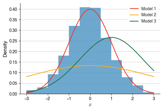
For my data (blue bars), which model (red, yellow, green lines), each with its own $$\theta$$, is the most likely one that generated the data?
Naturally, one can ask, what is the best $$\theta$$ for my observed data? This can be obtained by the likelihood function, which is the joint density of the data,
$$L(\theta) = \prod_{i=1}^{n} P(x_i\vert \theta)$$
This can start to get a bit confusing - why am I talking about $$\theta$$ and likelihoods? What does it have to do with Bayesian inference?
Philosophically speaking, our observed data is (often) a sample and the true value of $$\theta$$ is not known…
Bayesian Approach to Models
Frequentist statisticans try to deliver a point estimate of the model parameter(s), $$\theta$$. To quantify uncertainty around that estimate, standard error and/or confidence intervals are used (see this post for a good explanation).
$$\theta$$ is then estimated typically using maximum likelihood estimate (MLE) methods - either analytically (e.g. differentiating the log likelihood function), or numerically (e.g. using the expectation-maximisation algorithm).
Bayesian statisticans also agree that the true value of $$\theta$$ is fixed, but they express the uncertainty of their estimate of $$\theta$$ using distributions. The aim then is to derive the posterior distribution, $$P(\theta\vert x)$$, given some data and some prior belief about $$\theta$$ itself. In other words,
$$P(\theta\vert x) = \dfrac{P(x\vert \theta)P(\theta)}{P(x)}$$
What do these probabilities represent?
- $$P(\theta)$$ represents our prior belief about the parameter
- $$P(x\vert \theta)$$ represents our observations - evidence - or… likelihood!
- $$P(x)$$ is a normalising constant that represents the probability of $$x$$ irrespective of $$\theta$$.
Typically, $$P(x)$$ is difficult to calculate, so we represent the posterior being proportional to the product of the likelihood and the prior.
$$P(\theta\vert x) \propto P(x\vert \theta)P(\theta)$$
Santa Bayes at work
Let’s get to work! We can treat a child being naughty or nice as a binary variable, like a coin being heads or tails. Binary events like these are known as Bernoulli trials.
Thus, we can model the event of seeing a nice or naughty child as samples from a Bernoulli distribution.
$$x_i \sim \text{Bernoulli}(\theta)$$
At the crux of this is the rate of finding a naughty child, or $$\theta$$. This represents the parameter of our model which we want to estimate using Bayesian inference.
(From this point forth, a naughty child is represented by a 1, and good children by a 0).
# Let's see what Bernoulli-distributed variables look like.
# This is arbitrarily chosen for example reasons.
arbitrary_theta = 0.5

# Let's conduct 100 Bernoulli trials of our own, i.e., Santa visits 100 homes
np.random.seed(42)
children = [ i for i in bernoulli.rvs(size = 100, p = arbitrary_theta) ]

# Print the first 10
print(children[:10])
[0, 1, 1, 1, 0, 0, 0, 1, 1, 1]
Neat, so what happens when we change $$\theta$$?
## Plot the effects of bernoulli distribution parameters
fig, axes = plt.subplots(3, 2, sharey=True)
theta_init = 0.3
num_houses = 100

np.random.seed(42)
for i, ax in enumerate(axes.flatten()):

    theta = theta_init + 0.1 * i
    _obs = bernoulli.rvs(p = theta, size = num_houses)
    ax.bar([0, 1], [ (_obs==0).sum(), (_obs==1).sum() ], width = 0.5, label = "$\\theta$ = {:.1f}".format(theta))

    ax.set_xticks([0,1])
    ax.set_xticklabels(["Nice", "Naughty"])
    ax.legend()

fig.set_size_inches((6,6))
_ = fig.text(0.04, 0.5, "Number of naughty children", va = 'center', rotation = 90)
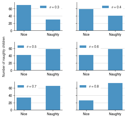
Depending on $$\theta$$, the number of naughty children changes; higher $$\theta$$ = more naughty kids!
While the frequentist is busy trying to derive the MLE for the likelihood function $$L(\theta)$$, the Bayesian creates yet another model describing the distribution of $$\theta$$, as we don’t know the true value of $$\theta$$.
In other words, Santa Bayes is uncertain about the true value of $$\theta$$. However, he can make an initial stab at $$\theta$$ - even if it isn’t hugely informative - and blend it with some observations to get an updated estimate of $$\theta$$.
This initial stab is what’s known as the prior distribution of $$\theta$$. Combined with some data, Santa will reach a new posterior distribution of $$\theta$$.
The choice of the prior can affect the shape of the posterior, but in practice, more observations (moar data) will
eventually swamp the effects of the prior.
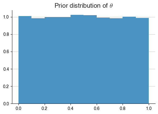
Knowing that our data - the distribution of naughty and nice children - follows a Bernoulli distribution, a suitable prior for $\theta$ is the uniform distribution.
There are several nice aspects of using a uniform prior for this problem:
- It makes very little assumptions on what the true value of $$\theta$$ can be
- It is very simple to implement!
Santa now decides to use a uniform prior for $$\theta$$, what does that look like?
# Initialise a pymc3 model
model = pm.Model()

with model:
    theta_dist = pm.Uniform("theta")

# Sample from the prior distribution of theta
rvs = theta_dist.random(size=20000)
bins = np.arange(0,1.01, 0.1)

h = plt.hist(rvs, density=True, bins = bins)
_ = plt.title("Prior distribution of $\\theta$")
With this prior distribution for $$\theta$$ in hand, Santa goes around the neighbourhood and checks for the number of naughty kids in the neighbourhood.
observations_test = [1]*13 + [0]*7 # 13 naughty kids, 7 nice ones, i.e. theta ~ 0.65
These observations can then be used for the likelihood function in pymc3. The key here is that we provide the Bernoulli likelihood function in pymc3 the set of observations. We also specify that the parameter for the Bernoulli distribution is sampled from the uniform prior that we have discussed earlier.
# Define a function to get the distribution of theta after MCMC
def get_trace(observations):

    # Initialise a pymc3 model
    model = pm.Model()

    with model:
        # This creates a distribution on theta
        theta_dist = pm.Uniform("theta")

        # Call the Bernoulli likelihood function observed_dist
        # The parameter for this distribution is from the prior, theta_dist;
        # observations are given to observed.
        observed_dist = pm.Bernoulli("obs", p = theta_dist, observed=observations)

        # Use the Metropolis-Hastings algorithm to estimate the posterior
        step = pm.Metropolis()
        trace = pm.sample(10000, step = step)

    return trace
In the function above, we use something called the Metropolis-Hastings algorithm to determine the posterior distribution. It’s a bit outside the scope of this post, but it’s essentially a technique that provides a numeric estimate of the true posterior distribution. It’s handy when you can’t derive an analytical solution.
trace = get_trace(observations=observations_test)

fig, ax = plt.subplots()

# MCMC methods have a burn-in period, so we discard the first few thousand iterations.
ax.hist(trace["theta"][2000:], density=True, bins = np.arange(0, 1.01, 0.05))
ax.axvline(13./20, linestyle = '--', color = 'k', label = '$\\theta$ estimated from relative frequency')
_ = ax.set_title("Posterior distribution of $\\theta$")
Multiprocess sampling (4 chains in 4 jobs)
Metropolis: [theta]
Sampling 4 chains, 0 divergences: 100%|██████████| 42000/42000 [00:08<00:00, 5162.22draws/s]
The number of effective samples is smaller than 25% for some parameters.
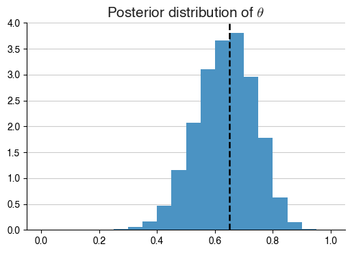
What’s happened here? Essentially, by giving a set of observations, we see that the posterior distribution of $$\theta$$ has been estimated, and it looks very different to our prior. In fact, it creates a bell curve-like histogram around $$\theta = 0.65$$.
Given this updated, posterior distribution of $$\theta$$, Santa can then do some calculations on this new distribution, such as:
- Summary statistics of the posterior distribution (mean, standard deviation)
- The maximum a posteriori estimate, or the MAP
- The 95% credible interval - not to be confused with confidence intervals!
Following these statistics, Santa can take further action on whether there are too many naughty kids in the neighbourhood, and whether it’s worth his time to stick around. Furthermore, Santa can use this updated posterior as a new prior for future inference activities.
In fact, we can see what happens when he goes to a different neighbourhood with a different number of nice kids, but with an identical uniform prior as before.
observations_nice = [1]*3 + [0]*17 # 9 naughty kids, 11 nice ones, i.e. theta ~ 0.15

trace = get_trace(observations=observations_nice)

fig, ax = plt.subplots()

# MCMC methods have a burn-in period, so we discard the first few thousand iterations.
ax.hist(trace["theta"][2000:], density=True, bins = np.arange(0, 1.01, 0.05))
ax.axvline(3./20, linestyle = '--', color = 'k', label = '$\\theta$ estimated from relative frequency')
_ = ax.set_title("Posterior distribution of $\\theta$")
Multiprocess sampling (4 chains in 4 jobs)
Metropolis: [theta]
Sampling 4 chains, 0 divergences: 100%|██████████| 42000/42000 [00:07<00:00, 5823.77draws/s]
The number of effective samples is smaller than 25% for some parameters.
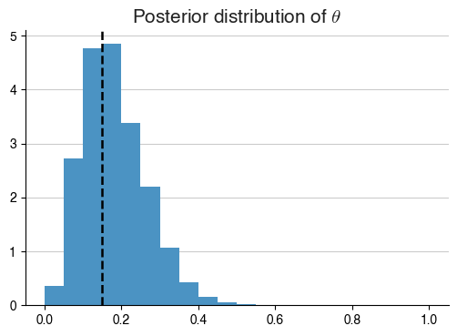
As we can see, for all intents and purposes, our implementation has remained almost identical, aside from the fact that our observation vectors are different. This leads to huge changes in the posterior distributions, and thus our understanding of $$\theta$$!
Effects of data size
OK, so now Santa has a framework for estimating the rate in which he’ll come across naughty or nice kids. How much will his posterior be affected by the number of observations?
For this example, we can generate some observations using a pre-defined, arbitrary $$\theta$$. We can then see if our posterior distribution converges to that arbitrary $$\theta$$ value, too.
arbitrary_theta = 0.2
small, medium, large = bernoulli.rvs(p=arbitrary_theta,size=10), bernoulli.rvs(p=arbitrary_theta,size=20),\
                       bernoulli.rvs(p=arbitrary_theta,size=200)

low_obs_trace = get_trace(small)
medium_trace = get_trace(medium)
high_obs_trace = get_trace(large)
Multiprocess sampling (4 chains in 4 jobs)
Metropolis: [theta]
Sampling 4 chains, 0 divergences: 100%|██████████| 42000/42000 [07:33<00:00, 92.67draws/s]
The number of effective samples is smaller than 25% for some parameters.
Multiprocess sampling (4 chains in 4 jobs)
Metropolis: [theta]
Sampling 4 chains, 0 divergences: 100%|██████████| 42000/42000 [00:07<00:00, 5564.29draws/s]
The number of effective samples is smaller than 25% for some parameters.
Multiprocess sampling (4 chains in 4 jobs)
Metropolis: [theta]
Sampling 4 chains, 0 divergences: 100%|██████████| 42000/42000 [00:07<00:00, 5974.85draws/s]
The number of effective samples is smaller than 25% for some parameters.
fig, ax = plt.subplots(1,3)

ax[0].hist(low_obs_trace["theta"][2000:], density=True, bins = np.arange(0, 1.01, 0.05))
ax[0].axvline(arbitrary_theta, linestyle = '--', color = 'k')
ax[0].set_title("Posterior $\\theta$ with 10 observations")

ax[1].hist(medium_trace["theta"][2000:], density=True, bins = np.arange(0, 1.01, 0.05))
ax[1].axvline(arbitrary_theta, linestyle = '--', color = 'k')
ax[1].set_title("Posterior $\\theta$ with 20 observations")

ax[2].hist(high_obs_trace["theta"][2000:], density=True, bins = np.arange(0, 1.01, 0.05))
ax[2].axvline(arbitrary_theta, linestyle = '--', color = 'k', label = 'Arbitrary $\\theta$')
ax[2].set_title("Posterior $\\theta$ with 200 observations")
ax[2].legend()

fig.set_size_inches((12,3))
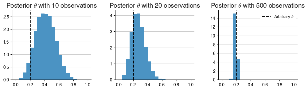
As we can see here, with more observations, we eventually diverge away from the shape of the prior. In fact, even from 10 observations, we can see that the posterior distribution of $$\theta$$ already looks dissimilar to the uniform prior we had specified before.
While the posterior distributions don’t converge tightly enough around the arbitrarily defined $$\theta$$ value unless there’s 500 observations, it’s clear that even with a small amount of data, we see positive results!
Effects of the prior
For the skeptic, we can choose a different prior distribution for $$\theta$$ - the Beta distribution:
$$\theta \sim \text{Beta}(\alpha, \beta)$$
The beta distribution, like the uniform distribution, is bound to values between 0 and 1. It is defined by two additional parameters, $$\alpha$$ and $$\beta$$. Thus, in this context, they are known as hyper-parameters for our use case.
Interestingly, the uniform distribution is a special case of the Beta distribution where $$\alpha = 1$$ and $$\beta = 1$$…
Does it matter what $$\alpha$$ and $$\beta$$ are?
def get_trace_beta(observations = None, alpha = 1, beta = 1):

    # Initialise a pymc3 model
    model = pm.Model()

    with model:
        theta_dist = pm.Beta("theta", alpha, beta)

        # Call the Bernoulli likelihood function obs
        # The parameter is from the prior, theta_dist
        # observations are given to observed.
        observed_dist = pm.Bernoulli("obs", p = theta_dist, observed=observations)

        # Use the Metropolis-Hastings algorithm
        step = pm.Metropolis()
        trace = pm.sample(10000, step = step)

    return theta_dist, trace
prior_a, hyper_a = get_trace_beta(small, alpha = 1, beta = 2)
prior_b, hyper_b = get_trace_beta(small, alpha = 2, beta = 2)
prior_c, hyper_c = get_trace_beta(small, alpha = 3, beta = 1)

prior_1, hyper_1 = get_trace_beta(large, alpha = 1, beta = 2)
prior_2, hyper_2 = get_trace_beta(large, alpha = 2, beta = 2)
prior_3, hyper_3 = get_trace_beta(large, alpha = 3, beta = 1)
fig, axes = plt.subplots(2,3, sharey=True)

ax = axes.flatten()

ax[0].hist(prior_a.random(size=20000), density=True, bins = np.arange(0, 1.01, 0.05), alpha = 0.4, label = "Prior")
ax[0].hist(hyper_a["theta"][2000:], density=True, bins = np.arange(0, 1.01, 0.05), alpha = 0.4, label = "Posterior")
ax[0].axvline(arbitrary_theta, linestyle = '--', color = 'k')
ax[0].set_title("$n = 10; \\alpha=1, \\beta=2$")

ax[1].hist(prior_b.random(size=20000), density=True, bins = np.arange(0, 1.01, 0.05), alpha = 0.4, label = "Prior")
ax[1].hist(hyper_b["theta"][2000:], density=True, bins = np.arange(0, 1.01, 0.05), alpha = 0.4, label = "Posterior")
ax[1].axvline(arbitrary_theta, linestyle = '--', color = 'k')
ax[1].set_title("$n = 10; \\alpha=2, \\beta=2$")

ax[2].hist(prior_c.random(size=20000), density=True, bins = np.arange(0, 1.01, 0.05), alpha = 0.4, label = "Prior")
ax[2].hist(hyper_c["theta"][2000:], density=True, bins = np.arange(0, 1.01, 0.05), alpha = 0.4, label = "Posterior")
ax[2].axvline(arbitrary_theta, linestyle = '--', color = 'k', label = 'Arbitrary $\\theta$')
ax[2].set_title("$n = 10; \\alpha=3, \\beta=1$")

ax[3].hist(prior_1.random(size=20000), density=True, bins = np.arange(0, 1.01, 0.05), alpha = 0.4, label = "Prior")
ax[3].hist(hyper_1["theta"][2000:], density=True, bins = np.arange(0, 1.01, 0.05), alpha = 0.4, label = "Posterior")
ax[3].axvline(arbitrary_theta, linestyle = '--', color = 'k')
ax[3].set_title("$n = 500; \\alpha=1, \\beta=2$")

ax[4].hist(prior_2.random(size=20000), density=True, bins = np.arange(0, 1.01, 0.05), alpha = 0.4, label = "Prior")
ax[4].hist(hyper_2["theta"][2000:], density=True, bins = np.arange(0, 1.01, 0.05), alpha = 0.4, label = "Posterior")
ax[4].axvline(arbitrary_theta, linestyle = '--', color = 'k')
ax[4].set_title("$n = 500; \\alpha=2, \\beta=2$")

ax[5].hist(prior_3.random(size=20000), density=True, bins = np.arange(0, 1.01, 0.05), alpha = 0.4, label = "Prior")
ax[5].hist(hyper_3["theta"][2000:], density=True, bins = np.arange(0, 1.01, 0.05), alpha = 0.4, label = "Posterior")
ax[5].axvline(arbitrary_theta, linestyle = '--', color = 'k', label = 'Arbitrary $\\theta$')
ax[5].set_title("$n = 500; \\alpha=3, \\beta=1$")
ax[5].legend()

fig.text(0.5, 0.04, "$\\theta$", ha = 'center')
fig.text(0.08, 0.5, "Density", va = 'center', rotation = 90)
fig.set_size_inches((12,6))
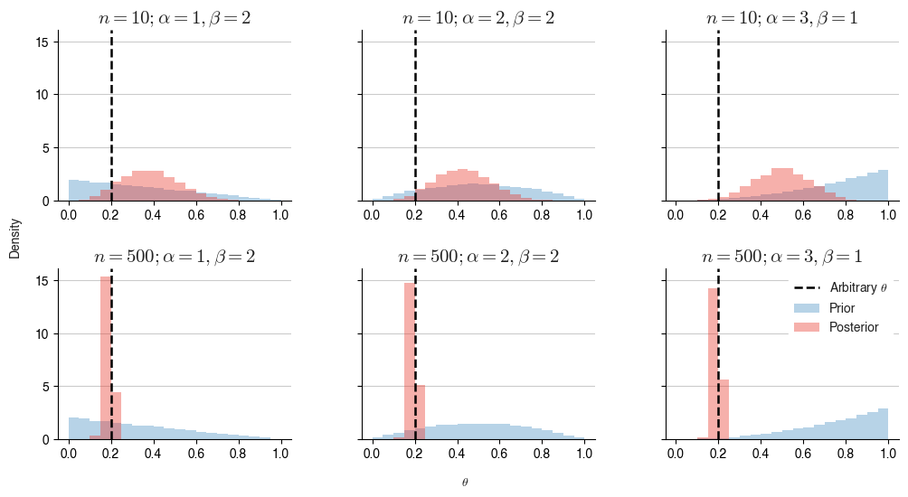
In short, when given identical observation vectors, the prior does still have an effect on the shape of the posterior, but it is clear that with a large number of observations, the data dominates the shape.
Final thoughts and Limitations
Enjoy reading this? :) I hope this was a nice intro to Bayesian inference! The take-aways really are:
- Bayesian inference is doable, but the learning curve is steep!
- Packages like pymc3 take away a lot of the leg-work, especially when your distributions aren’t mathematically nice to deal with.
- For real-world problems, they may not be as easily decomposable as we have in this example, but hopefully this gets you thinking about how Bayesians think about parameters in general.
- Conjugate priors and the details of MCMC haven’t been discussed but perhaps that’s for another time.
Here are some references I’ve come across and really benefited from when making this entry:
- Bayesian Methods for Hackers - hugely influential, I would say this formed a large chunk of my inspirations here.
- Bayesian Inference in One Hour - a solid set of lecutre notes from Patrick Lam.
- Refresher on Likelihood
- Some random SO / StackExchange threads, e.g. this one on credible intervals